
Should you wait for a cheaper flight? A gradient-boosting study of 94,000 fares
We trained gradient-boosted decision trees on three weeks of Wingman's fare checks. The model ranks coming price drops well (AUC 0.77–0.83), but no waiting policy beat buying at once.
Abstract
Should a traveller buy a fare now or wait for a lower one? We studied this question on Wingman's price log: 93,769 fare checks on 1,020 routes from 22 October to 12 November 2026. We set up two prediction tasks. The first task predicts whether the fare drops by 5 % or more within 3 days. The second task predicts how much a buyer saves by waiting. For both tasks, we trained gradient-boosted decision trees (LightGBM) and tested them on later days that the models never saw.
The drop model ranked drops well. Its ROC AUC was 0.77 to 0.83, against 0.67 to 0.71 for a baseline that uses only the days left before departure. But no policy built on the models saved money against buying at once. For flights more than a week away, the policies came out about even. So the Wingman app keeps its rule-based advice for now.
1. Data
Each time Wingman checks a watched trip, it writes the cheapest result of each search to a price log. A row holds:
- the time of the check, the two airports and the flight date
- the cheapest price, and the cheapest direct price when the result lists a direct flight
- the stops of the cheapest flight and the number of flights in the result
- the search settings: the stop limit, the currency, the travellers and the cabin
The log has no personal data.
We call the checks of one route, flight date, stop limit, travellers, cabin and currency a series. The log had 6,573 series. The median series has 6 checks, 10 % of the series have 20 or more, and the densest has 840. How often Wingman checks a series depends on the plan of the account that watches it and on the days left before departure. 93.5 % of the prices are in euros.
Densely checked series would fill the data set with near copies. So we kept at most one sample per series every 3 hours. This gave 54,896 samples.
2. The prediction tasks
Take a sample at time t with price p, and a horizon H of 3 days (7 days in a second test). Its window starts after t. The window ends at t + H or at the end of the flight date, whichever comes first.
Drop label. The label y is 1 when two checks in a row in the window both show a price of 0.95 p or less. Else y is 0. We ask for two checks so that a one-off blip in the results doesn't count as a drop.
Saving. We also measure what waiting gives a buyer: g = (p − p_wait) / p. If the window has a drop, p_wait is the higher price of the cheapest such pair of checks. A buyer who checks at either of the two times pays at most that price. Else, p_wait is the last price in the window. A positive g means that waiting saved money.
Censoring. We keep a sample only when its series has a check within 12 hours of the end of the window. Otherwise, the log doesn't show what happened. This left 35,253 samples with a 3-day label and 21,033 with a 7-day label.
3. Features
The models see 34 features. Each feature uses only checks at or before t, so no information from the future leaks in.
Table 1. The features. "÷" means "divided by".
| Group | Count | Features |
|---|---|---|
| Time | 6 | days left before departure, and its logarithm; weekday and month of the flight; hour and weekday of the check |
| Trip | 10 | distance between the airports (log); price in euros (log); travellers; cabin; checked bags; stop limit of the search; stops of the cheapest flight; direct flight listed; direct price ÷ cheapest price; flights listed (log) |
| Series: checks | 3 | earlier checks; age of the series; checks per day over the last 3 days |
| Series: price level | 5 | price ÷ the minimum, maximum, median and first price of the series; price at the minimum |
| Series: movement | 7 | price ÷ the price at the previous check, 24 hours ago and 72 hours ago; hours since the last change; over the last 7 days: share of checks with a change, price range ÷ median, number of 5 % steps down |
| Nearby dates | 3 | other flight dates within 7 days on the same route, checked in the last 3 days: their number; price ÷ their median; price ÷ their minimum |
4. The model
4.1 Gradient-boosted decision trees
A decision tree sorts samples with yes-or-no questions about one feature at a time, such as "are fewer than 9 days left?". Each leaf at the end holds a number. One small tree is a weak predictor. Gradient boosting adds many of them:
F(x) = f₁(x) + f₂(x) + … + f_M(x)
Each new tree f_m fits the negative gradient of the loss of the trees before it. So each tree corrects what the earlier trees still get wrong. A learning rate η scales each tree down, so that no single tree decides much (Friedman, 2001). For the drop label, the loss is the log loss, and the predicted probability is σ(F(x)) = 1 / (1 + e^(−F(x))).
We used LightGBM (Ke et al., 2017). It sorts the values of each feature into at most 255 bins before it looks for splits, which makes training fast. It grows each tree leaf by leaf: at each step, it splits the leaf that reduces the loss most. At each split, it also learns where samples with a missing value go. This matters here: a new series has no price from 72 hours ago, and the model can use that fact directly.
Trees suit this data. The features have different scales, some values are missing, and the effects interact. For example, a 5 % rise means one thing 3 days before departure and another thing 3 months before. A tree model handles all three without extra work. A neural network usually needs much more data than three weeks of prices.
4.2 Settings
We chose the settings before the first test and didn't tune them on the test data:
- 300 trees, with a learning rate η of 0.03
- at most 15 leaves per tree, and at least 40 samples per leaf
- each tree sees a random 80 % of the samples and 80 % of the features
- an L2 penalty of λ = 1 on the leaf values
Densely checked series give many samples that say nearly the same thing. So each sample gets the weight 1/√n, where n is the number of samples from its series.
4.3 Models of the saving
The drop model answers "will it drop?", but a buyer cares about money. So we trained two more LightGBM models on the saving g, with the same features and settings:
- Saving regression: predicts g, cut to ±30 %, with the Huber loss (δ = 0.05). This loss limits the effect of extreme values. The policy waits when the predicted saving is above 0.
- Cost-sensitive classifier: predicts whether g is above 0. Each sample also gets the weight |g| + 0.005, so that large savings and losses count most. The policy waits when the probability is 0.5 or more.
A third policy uses the drop model directly: wait when the probability of a drop is 0.5 or more.
4.4 Baselines
- Base rate: the share of drops in the training data, the same for every sample.
- Days to departure: the share of drops in the training data in five bands: 0–7, 8–21, 22–45, 46–90 and more than 90 days.
- Logistic regression: a linear model on the same 34 features, with an L2 penalty (C = 0.3). It replaces a missing value with the median and adds a yes-or-no feature for it. It scales each feature to a mean of 0 and a variance of 1.
5. Evaluation
Time split. A random split puts checks from the same days in the training set and in the test set. The test then looks better than real use. So we split by time, with a gap. For a cut-off date c, the training set has only the samples whose whole window ends before c (t + H ≤ c). The test set has the samples from c on. So no training label uses a price from after c.
For H = 3 days, we used three cut-offs: 1 November (with the test until 4 November), 3 November and 5 November. The test sets of the last two overlap. For H = 7 days, the log allowed one cut-off: 1 November.
Metrics. ROC AUC is the probability that a random sample with a drop gets a higher score than a random sample without one. 0.5 is chance, and 1 is perfect. The Brier score is the mean squared error of the predicted probability. The Brier skill score compares it with the Brier score of the base rate: 1 − BS / BS_base (Brier, 1950). A positive value means better probabilities than the base rate.
Intervals. Samples from one route aren't independent. So we resampled whole routes (a cluster bootstrap, 200 to 300 resamples) and give 90 % intervals.
Decision value. For each policy, we took the mean saving g per decision over the test set, with g = 0 when the policy buys at once. So buying at once scores 0. A policy with perfect foresight waits only when g is above 0, and gives the upper limit.
6. Results
6.1 Ranking drops
Table 2. ROC AUC for a drop within 3 days, with 90 % intervals.
| Cut-off | Days to departure | Logistic regression | LightGBM |
|---|---|---|---|
| 1 Nov (to 4 Nov) | 0.71 (0.65–0.76) | 0.77 (0.72–0.83) | 0.83 (0.80–0.86) |
| 3 Nov | 0.70 (0.68–0.72) | 0.71 (0.68–0.73) | 0.77 (0.75–0.79) |
| 5 Nov | 0.67 (0.65–0.70) | 0.73 (0.70–0.76) | 0.77 (0.75–0.80) |
The three test sets had 7,489, 18,558 and 13,586 samples, from 308, 596 and 588 routes. The share of drops was 7.6 to 9.0 % in the training sets and 11.6 to 16.3 % in the test sets.
LightGBM ranked drops best at every cut-off. At 7 days, with only 2,713 training samples, its AUC fell to 0.71 (0.67–0.74), and the AUC of logistic regression fell to 0.54.
In plain terms: show the model one sample with a coming drop and one without. It picks the right one about 8 times in 10.
6.2 Calibration
A model can rank well and still give wrong probabilities. The Brier skill score of LightGBM was only 1.4 to 4.7 %. The days-to-departure baseline did better, with 6.3 to 16.0 %. Table 3 shows why.
Table 3. The drop probability that LightGBM predicted, against the real share of drops, by fifths of the test set (cut-off 3 November).
| Fifth of the test set | Mean prediction | Real share of drops |
|---|---|---|
| 1 (lowest) | 0.5 % | 2.0 % |
| 2 | 2.1 % | 4.8 % |
| 3 | 7.6 % | 12.5 % |
| 4 | 24.2 % | 21.4 % |
| 5 (highest) | 62.9 % | 35.7 % |
The predictions are too low at the bottom and too high at the top. The share of drops almost doubled from the training days to the test days (8.2 % to 15.3 %), so the base level moved. At the top, the model is too sure of itself. Calibration on recent data, for example with isotonic regression, could correct part of this. But calibration needs its own slice of recent data, and three weeks don't give enough.
6.3 What the model uses
The split gain of the drop model shows which features it uses most:
- days left before departure: 30 % (in two forms, 22.5 % and 7.3 %)
- the price in euros: 7.8 %
- the price divided by the cheapest nearby date: 7.1 %
- the number of earlier checks: 7.1 %
- the distance: 6.8 %
- the stop limit of the search: 6.3 %
Two things stand out. First, the recent trend ranks low: the change since the previous check, or since 24 or 72 hours ago. A fall or a rise in the last days says little about the next days. Second, the number of earlier checks ranks high. A series that Wingman checks often has more chances to show two low checks in a row. So part of what the model learns is how often Wingman checks a flight, not only how its price behaves.
6.4 Decision value
Table 4. Mean saving per decision against buying at once: 3-day horizon, all test samples, 90 % intervals. A negative value means that the policy paid more.
| Policy | 1 Nov (to 4 Nov) | 3 Nov | 5 Nov |
|---|---|---|---|
| Buy at once | 0 | 0 | 0 |
| Always wait | −3.5 % (−5.3 to −2.1) | −5.7 % (−7.2 to −4.0) | −5.3 % (−7.1 to −3.8) |
| Drop model, wait if P ≥ 0.5 | −1.5 % (−2.9 to −0.4) | −2.7 % (−3.9 to −1.7) | −0.6 % (−1.2 to −0.1) |
| Saving regression | −1.9 % (−3.4 to −0.5) | −0.6 % (−1.2 to −0.1) | −0.7 % (−1.3 to −0.1) |
| Cost-sensitive classifier | −0.7 % (−2.1 to +0.4) | −2.1 % (−3.2 to −1.0) | −0.3 % (−0.8 to +0.2) |
| Perfect foresight | +2.8 % | +2.9 % | +3.0 % |
No policy beat buying at once. The drop model was right in 41 to 47 % of its "wait" decisions, but a wrong wait cost more than a right wait saved. Waiting 7 days was worse: always waiting cost 14.6 % on average, and the drop-model policy cost 5.2 %.
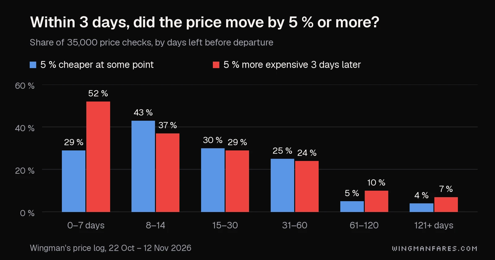
Most of the loss comes from the last week before departure. Figure 1, at the top of this post, shows how often a price moved by 5 % or more within 3 days. In the last 7 days, the price was 5 % higher three days later in 52 % of the samples, and it dropped in only 29 %. From 8 to 60 days out, drops and rises came about equally often, each in 24 to 43 % of the samples. More than 60 days out, only 4 to 5 % of the prices dropped within 3 days.
So we ran the test again without the last week: only flights more than 7 days away. Always waiting then cost 0.6 to 1.5 % at 3 days and 1.9 to 2.3 % at 7 days. Over the 5 test periods and the 3 policies, the model policies landed between −1.3 % and +0.5 % per decision.
One of these 15 intervals lay above zero: the cost-sensitive classifier at 3 days and cut-off 1 November, with +0.5 % (+0.2 to +0.9). With 15 comparisons, one such interval is likely by chance. The same policy also lost money at the other two 3-day cut-offs. We read the result as "about even", and that isn't enough to tell anyone to wait.
7. Limitations
- Short span. Three weeks show no seasons. The training and test days already differed: the share of drops almost doubled.
- Selection. The routes are the ones that Wingman users watch. Most of them start in Europe, and 93.5 % of the prices are in euros. Other routes and other months can behave differently.
- Irregular checks. The log sees a price only when Wingman checks it. A drop between two checks is invisible, and the label depends on how often Wingman checks a series.
- The waiting buyer. The saving assumes that a waiting buyer sees the drop. That needs a check while the drop lasts, and many drops are short.
- Correlated samples. The route bootstrap handles part of the dependence between samples. The real uncertainty can still be larger than our intervals.
- No tuning. We chose the settings in advance. Tuning could help a little, but it needs its own validation period.
- No direct comparison with the app. The app's buy-or-wait rules also use a monthly reference price for each route. The log doesn't store it, so we couldn't run the rules fairly on these samples.
8. Related work
Etzioni et al. (2003) asked the same question with fares that they collected for two routes in the United States. They found that a learned policy could save money against buying at once. Groves and Gini (2013) studied more routes and chose the features automatically. Both studies followed few routes over a longer time. Our data is the other way round: many routes over a short time. We think that the short time is the main reason why our models don't pay yet.
9. Conclusion and next steps
The drop model ranks well, but it doesn't yet give a buyer a way to save money. So the Wingman app keeps its buy-or-wait rules for now. The rules use the usual price for the route, the history of the watch and the days left before departure.
Next steps:
- More data. The log keeps a year of prices. In December, with two months of data, we'll run the same test again.
- A stricter bar. A model goes into the app only when one of its policies beats buying at once at more than one cut-off. Its interval must also lie above zero.
- A new target. We'll also try to predict the lowest price before departure directly, as a quantile.
- A second use. The ranking already works. Wingman could check the flights with a high chance of a drop more often, and so catch more drops with the same number of searches.
For travellers, the data supports three simple rules:
- In the last week, book when you see a price you can accept.
- One to two months out, a price can go either way. Wait only if something watches the price for you.
- Months out, prices change slowly. You don't need to check them every day.
References
- Brier, G. W. (1950). Verification of forecasts expressed in terms of probability. Monthly Weather Review, 78(1), 1–3.
- Etzioni, O., Tuchinda, R., Knoblock, C. A., and Yates, A. (2003). To buy or not to buy: mining airfare data to minimize ticket purchase price. Proceedings of the 9th ACM SIGKDD International Conference on Knowledge Discovery and Data Mining.
- Friedman, J. H. (2001). Greedy function approximation: a gradient boosting machine. Annals of Statistics, 29(5), 1189–1232.
- Groves, W., and Gini, M. (2013). Optimal airline ticket purchasing using automated user-guided feature selection. Proceedings of the 23rd International Joint Conference on Artificial Intelligence (IJCAI).
- Ke, G., Meng, Q., Finley, T., Wang, T., Chen, W., Ma, W., Ye, Q., and Liu, T.-Y. (2017). LightGBM: a highly efficient gradient boosting decision tree. Advances in Neural Information Processing Systems 30.